FLIM Analysis

In this example we will use SciJava Ops within Fiji to perform FLIM analysis, which is used in many situations including photosensitizer detection and FRET measurement.

We use a sample of FluoCells™ Prepared Slide #1, imaged by Jenu Chacko using Openscan-LSM and SPC180 electronics with multiphoton excitation and a 40x WI lens. Notably, the full field for this image is 130 microns in each axial dimension.

FluoCells™ Prepared Slide #1 contains bovine pulmonary artery endothelial cells (BPAEC). MitoTracker™ Red CMXRos was used to stain the mitochondria in the live cells, with accumulation dependent upon membrane potential. Following fixation and permeabilization, F-actin was stained with Alexa Fluor™ 488 phalloidin, and the nuclei were counterstained with the blue-fluorescent DNA stain DAPI.

The sample data can be downloaded here and can be loaded into Fiji with Bio-Formats using File → Open. When presented with the Bio-Formats Import Options screen, it may be helpful to select Metadata viewing → Display metadata to determine values necessary for analysis. Then, select OK. The data may take a minute to load.

Within the script, the Levenberg-Marquardt algorithm fitting Op of SciJava Ops FLIM is used to fit the data.

Basic analysis

Script execution requires a number of parameters, which may be useful for adapting this script to other datasets. For this dataset, we use the following values:

Parameter	Value
Time Base	12.5
Time Bins	256
Lifetime Axis	2
Intensity Threshold	18
Bin Kernel Radius	1

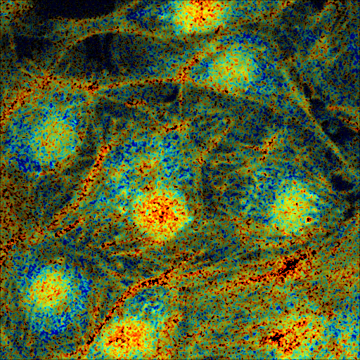
The script above will display the fit results, as well as a pseudocolored output image. The results are shown in the panels below, and are described from left to right:

• The first initial fluorescence parameter A₁

• The first fluorescence lifetime τ₁ (contrasted using ImageJ’s B&C plugin (Ctrl + Shift + C), by selecting the Set option and providing 0 as the minimum and 3 as the maximum).

• The pseudocolored result, an HSV image where

  • Hue and Saturation are a function of τ₁, where the function is a LUT provided optionally by the user. The LUT used by TRI2 is used by default, and is also used explicitly in this use case.

  • Value is a function of A₁

Additionally, the script outputs tLow and tHigh, Doubles describing the 5th and 95th percentiles respectively, across all τ₁. Lifetime parameters outside of the range [tLow, tHigh] are clipped to the nearest bound in the pseudocolored image.

Result	Value
tLow	1.87000572681427
tHigh	2.3314802646636963

The pseudocolored result shows a clear separation of fluorophores, which could be segmented and further processed.

Groovy

#@ OpEnvironment ops
#@ ROIService roiService
#@ Img input
#@ Float (description="The total time (ns) (timeBase in metadata)", label = "Time Base", value=12.5) timeBase
#@ Integer (description="The number of time bins (timeBins in metadata)", label = "Time Bins", value=512) timeBins
#@ Integer (description="The index of the lifetime axis (from metadata)", label = "Lifetime Axis", value=2) lifetimeAxis
#@ Float (description="The minimal pixel intensity (across all time bins) threshold for fitting", label = "Intensity Threshold", value = 18) iThresh
#@ Integer (description="The radius of the binning kernel", label = "Bin Kernel Radius", value=1, min=0) kernelRad
#@OUTPUT Img A1
#@OUTPUT Img Tau1
#@OUTPUT Img pseudocolored
#@OUTPUT Double tLow
#@OUTPUT Double tHigh

import java.lang.System
import net.imglib2.roi.Regions
import net.imglib2.type.numeric.real.DoubleType

import org.scijava.ops.flim.FitParams
import org.scijava.ops.flim.Pseudocolor

// Utility function to collapse all ROIs into a single mask for FLIM fitting
def getMask() {
    // No ROIs
    if (!roiService.hasROIs(input)) {
        return null
    }
    // 1+ ROIs
    rois = roiService.getROIs(input)
    mask = rois.children()remove(0).data()
    for(roi: rois.children()) {
        mask = mask.or(roi.data())
    }
    return mask;
}

def getPercentile(img, mask, percentile) {
    if (mask != null) {
        img = Regions.sampleWithRealMask(mask, img)
    }
    return ops.op("stats.percentile")
        .input(img, percentile)
        .outType(DoubleType.class)
        .apply()
        .getRealFloat()
}

start = System.currentTimeMillis()

// The FitParams contain a set of reasonable defaults for FLIM curve fitting
param = new FitParams()
param.transMap = input
param.ltAxis = lifetimeAxis
param.iThresh = iThresh
// xInc is the difference (ns) between two bins
param.xInc = timeBase / timeBins

// Fit curves
kernel = ops.op("create.kernelSum").input(1 + 2 * kernelRad).apply()
lma = ops.op("flim.fitLMA").input(param, getMask(), kernel).apply()

// The fit results paramMap is a XYC image, with result attributes along the Channel axis
fittedImg = lma.paramMap
// For LMA, we have Z, A1, and Tau1 as the three attributes
A1 = ops.op("transform.hyperSliceView").input(fittedImg, lifetimeAxis, 1).apply()
Tau1 = ops.op("transform.hyperSliceView").input(fittedImg, lifetimeAxis, 2).apply()

// Finally, generate a pseudocolored result
tLow = getPercentile(Tau1, mask, 5.0)
tHigh = getPercentile(Tau1, mask, 95.0)
pseudocolored = ops.op("flim.pseudocolor").input(lma, tLow, tHigh, null, null, Pseudocolor.tri2()).apply()

end = System.currentTimeMillis()
println("Finished fitting in " + (end - start) + " milliseconds")

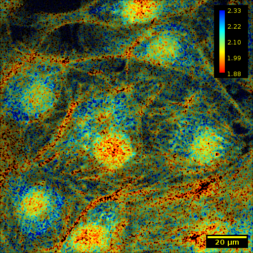
Adding Calibration and Scale Bars

To attach quantitative meaning to the pseudocolored image, we must add calibration and scale bars. We add each within ImageJ using a second SciJava script using the following parameters. Note that tLow and tHigh are outputs from the previous script.

With 130 microns across each direction in the dataset, we have 512/130~3.938 pixels per micron.

Parameter	Value
tLow	1.87000572681427
tHigh	2.3314802646636963
Pixels Per Micron	3.938461538

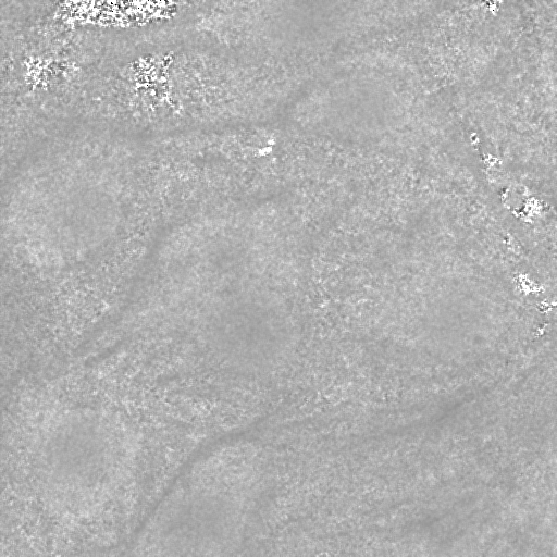
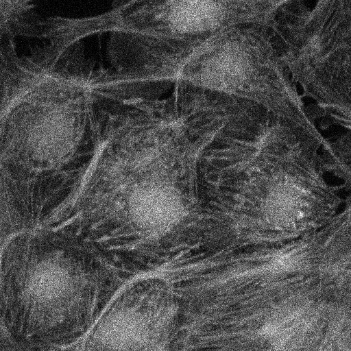
The results are shown in the panels below. The left panel shows panel 56 of the original image, contrasted using ImageJ’s Brightness and Contrast tool, and the right panel shows the annotated, pseudocolored results.

Groovy

#@ ImagePlus Tau1
#@ ImagePlus pseudocolored
#@ Double (description="Lower bound of clip range in Tau1", label = "Tau Low", value = 1.87000572681427) tLow
#@ Double (description="Upper bound of clip range in Tau1", label = "Tau High", value = 2.3314802646636963) tHigh
#@ Double (description="The number of pixels per micron", label = "Pixels per Micron", value = 3.938461538) ppm

import org.scijava.ops.flim.Pseudocolor
import ij.process.LUT
import ij.IJ

// The pseudocolored image uses lifetime values between tLow and tHigh
// for an accurate calibration bar, we must also restrict display
// values to that range.
Tau1 = Tau1.clone()
Tau1.setDisplayRange(tLow, tHigh)

// Set the LUT & Calibration Bar
rgb = Pseudocolor.tri2().getValues()
lut = new LUT(rgb[0], rgb[1], rgb[2])
Tau1.setLut(lut)
IJ.run(Tau1, "Calibration Bar...", "location=[Upper Right] fill=Black label=Yellow number=5 decimal=2 font=12 zoom=1 overlay");

// Set the scale & Scale Bar
IJ.run(Tau1, "Set Scale...", "distance=" + ppm + " known=1 unit=µm");
IJ.run(Tau1, "Scale Bar...", "width=20 height=20 color=Yellow background=Black horizontal bold overlay");
// Finally, copy the Overlay over to the pseudocolored image
pseudocolored.setOverlay(Tau1.getOverlay())

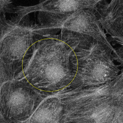
Subsampling Within ROIs

Curve fitting can be an intensive process, requiring significant resources to process larger datasets. For this reason, there can be significant benefit in restricting computation to Regions of Interest (ROIs), and SciJava Ops FLIM allows ROIs to restrict computation for all fitting Ops.

The provided script allows users to specify ROIs by drawing selections using the ImageJ UI. These selections are converted to ImgLib2 RealMask objects, which are then optionally passed to the Op.

In the panels below, we show the results of executing both scripts with computation restricted to the area around a single cell. The left panel shows slide 56 of the input data, annotated with an elliptical ROI drawn using ImageJ’s elliptical selection tool and contrasted using ImageJ’s Brightness and Contrast tool. The right panel shows the pseudocolored result, annotated with color and scale bars, with computation limited to the selected ellipse.